Strain Small
Displacement Large
Material Linear elastic
In the Total Lagrangian formulation, the initial undeformed configuration is the reference configuration. All derivatives, Jacobians and volume integrals are evaluated with respect to that initial configuration. The development follows Section 12.2 ; the HEX8 interpolation and linear formulation are presented in Section 25.1 .
01
Strain and stress notation The Green–Lagrange strain vector and the corresponding stress vector are:
ε = { ε x ε y ε z γ x y γ y z γ z x } , σ = { σ x σ y σ z τ x y τ y z τ z x } . \htmlClass{fea-math-bold-italic}{\boldsymbol{\varepsilon}}=\begin{Bmatrix}\varepsilon_x\\\varepsilon_y\\\varepsilon_z\\\gamma_{xy}\\\gamma_{yz}\\\gamma_{zx}\end{Bmatrix},\qquad\htmlClass{fea-math-bold-italic}{\boldsymbol{\sigma}}=\begin{Bmatrix}\sigma_x\\\sigma_y\\\sigma_z\\\tau_{xy}\\\tau_{yz}\\\tau_{zx}\end{Bmatrix}. ε = ⎩ ⎨ ⎧ ε x ε y ε z γ x y γ y z γ z x ⎭ ⎬ ⎫ , σ = ⎩ ⎨ ⎧ σ x σ y σ z τ x y τ y z τ z x ⎭ ⎬ ⎫ . Remark. In this section the symbol ε \htmlClass{fea-math-bold-italic}{\boldsymbol{\varepsilon}} ε σ \htmlClass{fea-math-bold-italic}{\boldsymbol{\sigma}} σ
σ = D ε . \htmlClass{fea-math-bold-italic}{\boldsymbol{\sigma}}=\htmlClass{fea-math-bold-italic}{\boldsymbol D}\htmlClass{fea-math-bold-italic}{\boldsymbol{\varepsilon}}. σ = D ε . This notation simplifies the transition from the linear formulation while preserving the Total Lagrangian character of the analysis.
D = E ( 1 − ν ) ( 1 + ν ) ( 1 − 2 ν ) [ 1 ν 1 − ν ν 1 − ν 0 0 0 ν 1 − ν 1 ν 1 − ν 0 0 0 ν 1 − ν ν 1 − ν 1 0 0 0 0 0 0 1 − 2 ν 2 ( 1 − ν ) 0 0 0 0 0 0 1 − 2 ν 2 ( 1 − ν ) 0 0 0 0 0 0 1 − 2 ν 2 ( 1 − ν ) ] . \htmlClass{fea-math-bold-italic}{\boldsymbol D}=\frac{E(1-\nu)}{(1+\nu)(1-2\nu)}\begin{bmatrix}1&\frac\nu{1-\nu}&\frac\nu{1-\nu}&0&0&0\\\frac\nu{1-\nu}&1&\frac\nu{1-\nu}&0&0&0\\\frac\nu{1-\nu}&\frac\nu{1-\nu}&1&0&0&0\\0&0&0&\frac{1-2\nu}{2(1-\nu)}&0&0\\0&0&0&0&\frac{1-2\nu}{2(1-\nu)}&0\\0&0&0&0&0&\frac{1-2\nu}{2(1-\nu)}\end{bmatrix}. D = ( 1 + ν ) ( 1 − 2 ν ) E ( 1 − ν ) 1 1 − ν ν 1 − ν ν 0 0 0 1 − ν ν 1 1 − ν ν 0 0 0 1 − ν ν 1 − ν ν 1 0 0 0 0 0 0 2 ( 1 − ν ) 1 − 2 ν 0 0 0 0 0 0 2 ( 1 − ν ) 1 − 2 ν 0 0 0 0 0 0 2 ( 1 − ν ) 1 − 2 ν . 02
Deformation energy The deformation energy is evaluated over the initial element volumes:
U = 1 2 ∑ e l = 1 n e l ∫ V 0 e l ε T σ d V 0 . U=\frac12\sum_{el=1}^{n_{el}}\int_{V_{0el}}\htmlClass{fea-math-bold-italic}{\boldsymbol{\varepsilon}}^T\htmlClass{fea-math-bold-italic}{\boldsymbol{\sigma}}\,dV_0. U = 2 1 e l = 1 ∑ n e l ∫ V 0 e l ε T σ d V 0 . Here V 0 e l V_{0el} V 0 e l n e l n_{el} n e l s , t , r s,t,r s , t , r
U = 1 2 ∑ e l = 1 n e l ∫ − 1 1 ∫ − 1 1 ∫ − 1 1 ε ( s , t , r ) T σ ( s , t , r ) d e t ( J 0 ( s , t , r ) ) d s d t d r . U=\frac12\sum_{el=1}^{n_{el}}\int_{-1}^{1}\int_{-1}^{1}\int_{-1}^{1}\htmlClass{fea-math-bold-italic}{\boldsymbol{\varepsilon}}(s,t,r)^T\htmlClass{fea-math-bold-italic}{\boldsymbol{\sigma}}(s,t,r)\mathop{\mathit{det}}\!\big(\htmlClass{fea-math-bold-italic}{\boldsymbol J}_0(s,t,r)\big)\,ds\,dt\,dr. U = 2 1 e l = 1 ∑ n e l ∫ − 1 1 ∫ − 1 1 ∫ − 1 1 ε ( s , t , r ) T σ ( s , t , r ) det ( J 0 ( s , t , r ) ) d s d t d r . 03
Jacobian and interpolation derivatives As in Section 25.1 , the Jacobian is obtained from the interpolation derivatives and the nodal coordinates:
J 0 ( s , t , r ) = [ x , s y , s z , s x , t y , t z , t x , r y , r z , r ] = H ( s , t , r ) x e l , x e l = [ x 1 y 1 z 1 x 2 y 2 z 2 x 3 y 3 z 3 x 4 y 4 z 4 x 5 y 5 z 5 x 6 y 6 z 6 x 7 y 7 z 7 x 8 y 8 z 8 ] . \htmlClass{fea-math-bold-italic}{\boldsymbol J}_0(s,t,r)=\begin{bmatrix}x_{,s}&y_{,s}&z_{,s}\\x_{,t}&y_{,t}&z_{,t}\\x_{,r}&y_{,r}&z_{,r}\end{bmatrix}=\htmlClass{fea-math-bold-italic}{\boldsymbol H}(s,t,r)\htmlClass{fea-math-bold-italic}{\boldsymbol x}_{el},\qquad\htmlClass{fea-math-bold-italic}{\boldsymbol x}_{el}=\begin{bmatrix}x_1&y_1&z_1\\x_2&y_2&z_2\\x_3&y_3&z_3\\x_4&y_4&z_4\\x_5&y_5&z_5\\x_6&y_6&z_6\\x_7&y_7&z_7\\x_8&y_8&z_8\end{bmatrix}. J 0 ( s , t , r ) = x , s x , t x , r y , s y , t y , r z , s z , t z , r = H ( s , t , r ) x e l , x e l = x 1 x 2 x 3 x 4 x 5 x 6 x 7 x 8 y 1 y 2 y 3 y 4 y 5 y 6 y 7 y 8 z 1 z 2 z 3 z 4 z 5 z 6 z 7 z 8 . x i , y i , z i x_i,y_i,z_i x i , y i , z i
H ( s , t , r ) = 1 8 [ ( 1 + t ) ( 1 + r ) − ( 1 + t ) ( 1 + r ) − ( 1 − t ) ( 1 + r ) ( 1 − t ) ( 1 + r ) ( 1 + t ) ( 1 − r ) − ( 1 + t ) ( 1 − r ) − ( 1 − t ) ( 1 − r ) ( 1 − t ) ( 1 − r ) ( 1 + s ) ( 1 + r ) ( 1 − s ) ( 1 + r ) − ( 1 − s ) ( 1 + r ) − ( 1 + s ) ( 1 + r ) ( 1 + s ) ( 1 − r ) ( 1 − s ) ( 1 − r ) − ( 1 − s ) ( 1 − r ) − ( 1 + s ) ( 1 − r ) ( 1 + s ) ( 1 + t ) ( 1 − s ) ( 1 + t ) ( 1 − s ) ( 1 − t ) ( 1 + s ) ( 1 − t ) − ( 1 + s ) ( 1 + t ) − ( 1 − s ) ( 1 + t ) − ( 1 − s ) ( 1 − t ) − ( 1 + s ) ( 1 − t ) ] . \htmlClass{fea-math-bold-italic}{\boldsymbol H}(s,t,r)=\frac18\begin{bmatrix}(1+t)(1+r)&-(1+t)(1+r)&-(1-t)(1+r)&(1-t)(1+r)&(1+t)(1-r)&-(1+t)(1-r)&-(1-t)(1-r)&(1-t)(1-r)\\(1+s)(1+r)&(1-s)(1+r)&-(1-s)(1+r)&-(1+s)(1+r)&(1+s)(1-r)&(1-s)(1-r)&-(1-s)(1-r)&-(1+s)(1-r)\\(1+s)(1+t)&(1-s)(1+t)&(1-s)(1-t)&(1+s)(1-t)&-(1+s)(1+t)&-(1-s)(1+t)&-(1-s)(1-t)&-(1+s)(1-t)\end{bmatrix}. H ( s , t , r ) = 8 1 ( 1 + t ) ( 1 + r ) ( 1 + s ) ( 1 + r ) ( 1 + s ) ( 1 + t ) − ( 1 + t ) ( 1 + r ) ( 1 − s ) ( 1 + r ) ( 1 − s ) ( 1 + t ) − ( 1 − t ) ( 1 + r ) − ( 1 − s ) ( 1 + r ) ( 1 − s ) ( 1 − t ) ( 1 − t ) ( 1 + r ) − ( 1 + s ) ( 1 + r ) ( 1 + s ) ( 1 − t ) ( 1 + t ) ( 1 − r ) ( 1 + s ) ( 1 − r ) − ( 1 + s ) ( 1 + t ) − ( 1 + t ) ( 1 − r ) ( 1 − s ) ( 1 − r ) − ( 1 − s ) ( 1 + t ) − ( 1 − t ) ( 1 − r ) − ( 1 − s ) ( 1 − r ) − ( 1 − s ) ( 1 − t ) ( 1 − t ) ( 1 − r ) − ( 1 + s ) ( 1 − r ) − ( 1 + s ) ( 1 − t ) . The Cartesian derivatives of the interpolation functions are collected in:
b = J 0 − 1 H = [ b 11 b 12 b 13 b 14 b 15 b 16 b 17 b 18 b 21 b 22 b 23 b 24 b 25 b 26 b 27 b 28 b 31 b 32 b 33 b 34 b 35 b 36 b 37 b 38 ] . \htmlClass{fea-math-bold-italic}{\boldsymbol b}=\htmlClass{fea-math-bold-italic}{\boldsymbol J}_0^{-1}\htmlClass{fea-math-bold-italic}{\boldsymbol H}=\begin{bmatrix}b_{11}&b_{12}&b_{13}&b_{14}&b_{15}&b_{16}&b_{17}&b_{18}\\b_{21}&b_{22}&b_{23}&b_{24}&b_{25}&b_{26}&b_{27}&b_{28}\\b_{31}&b_{32}&b_{33}&b_{34}&b_{35}&b_{36}&b_{37}&b_{38}\end{bmatrix}. b = J 0 − 1 H = b 11 b 21 b 31 b 12 b 22 b 32 b 13 b 23 b 33 b 14 b 24 b 34 b 15 b 25 b 35 b 16 b 26 b 36 b 17 b 27 b 37 b 18 b 28 b 38 . b \htmlClass{fea-math-bold-italic}{\boldsymbol b} b b 1 i = N i , x , b 2 i = N i , y , b 3 i = N i , z b_{1i}=N_{i,x},\ b_{2i}=N_{i,y},\ b_{3i}=N_{i,z} b 1 i = N i , x , b 2 i = N i , y , b 3 i = N i , z
04
Green–Lagrange strains The full three-dimensional Green–Lagrange strain expressions are:
ε x = u , x + 1 2 ( u , x 2 + v , x 2 + w , x 2 ) , ε y = v , y + 1 2 ( u , y 2 + v , y 2 + w , y 2 ) , ε z = w , z + 1 2 ( u , z 2 + v , z 2 + w , z 2 ) , γ x y = u , y + v , x + u , x u , y + v , x v , y + w , x w , y , γ y z = v , z + w , y + u , y u , z + v , y v , z + w , y w , z , γ z x = w , x + u , z + u , z u , x + v , z v , x + w , z w , x . \begin{aligned}\varepsilon_x&=u_{,x}+\tfrac12(u_{,x}^2+v_{,x}^2+w_{,x}^2),\\\varepsilon_y&=v_{,y}+\tfrac12(u_{,y}^2+v_{,y}^2+w_{,y}^2),\\\varepsilon_z&=w_{,z}+\tfrac12(u_{,z}^2+v_{,z}^2+w_{,z}^2),\\\gamma_{xy}&=u_{,y}+v_{,x}+u_{,x}u_{,y}+v_{,x}v_{,y}+w_{,x}w_{,y},\\\gamma_{yz}&=v_{,z}+w_{,y}+u_{,y}u_{,z}+v_{,y}v_{,z}+w_{,y}w_{,z},\\\gamma_{zx}&=w_{,x}+u_{,z}+u_{,z}u_{,x}+v_{,z}v_{,x}+w_{,z}w_{,x}.\end{aligned} ε x ε y ε z γ x y γ y z γ z x = u , x + 2 1 ( u , x 2 + v , x 2 + w , x 2 ) , = v , y + 2 1 ( u , y 2 + v , y 2 + w , y 2 ) , = w , z + 2 1 ( u , z 2 + v , z 2 + w , z 2 ) , = u , y + v , x + u , x u , y + v , x v , y + w , x w , y , = v , z + w , y + u , y u , z + v , y v , z + w , y w , z , = w , x + u , z + u , z u , x + v , z v , x + w , z w , x . A comma denotes differentiation with respect to an initial Cartesian coordinate, for example u , x = ∂ u / ∂ x u_{,x}=\partial u/\partial x u , x = ∂ u / ∂ x
u e l = { u 1 v 1 w 1 u 2 v 2 w 2 ⋯ u 8 v 8 w 8 } T . \htmlClass{fea-math-bold-italic}{\boldsymbol u}_{el}=\begin{Bmatrix}u_1&v_1&w_1&u_2&v_2&w_2&\cdots&u_8&v_8&w_8\end{Bmatrix}^T. u e l = { u 1 v 1 w 1 u 2 v 2 w 2 ⋯ u 8 v 8 w 8 } T . Following Section 12.2 , the displacement derivatives are written as:
u , x = B u x u e l , u , y = B u y u e l , u , z = B u z u e l v , x = B v x u e l , v , y = B v y u e l , v , z = B v z u e l w , x = B w x u e l , w , y = B w y u e l , w , z = B w z u e l \begin{aligned}u_{,x}&=\htmlClass{fea-math-bold-italic}{\boldsymbol{B}}_{u_x}\htmlClass{fea-math-bold-italic}{\boldsymbol{u}}_{el},\qquad u_{,y}&=\htmlClass{fea-math-bold-italic}{\boldsymbol{B}}_{u_y}\htmlClass{fea-math-bold-italic}{\boldsymbol{u}}_{el},\qquad u_{,z}&=\htmlClass{fea-math-bold-italic}{\boldsymbol{B}}_{u_z}\htmlClass{fea-math-bold-italic}{\boldsymbol{u}}_{el}\\v_{,x}&=\htmlClass{fea-math-bold-italic}{\boldsymbol{B}}_{v_x}\htmlClass{fea-math-bold-italic}{\boldsymbol{u}}_{el},\qquad v_{,y}&=\htmlClass{fea-math-bold-italic}{\boldsymbol{B}}_{v_y}\htmlClass{fea-math-bold-italic}{\boldsymbol{u}}_{el},\qquad v_{,z}&=\htmlClass{fea-math-bold-italic}{\boldsymbol{B}}_{v_z}\htmlClass{fea-math-bold-italic}{\boldsymbol{u}}_{el}\\w_{,x}&=\htmlClass{fea-math-bold-italic}{\boldsymbol{B}}_{w_x}\htmlClass{fea-math-bold-italic}{\boldsymbol{u}}_{el},\qquad w_{,y}&=\htmlClass{fea-math-bold-italic}{\boldsymbol{B}}_{w_y}\htmlClass{fea-math-bold-italic}{\boldsymbol{u}}_{el},\qquad w_{,z}&=\htmlClass{fea-math-bold-italic}{\boldsymbol{B}}_{w_z}\htmlClass{fea-math-bold-italic}{\boldsymbol{u}}_{el}\\\end{aligned} u , x v , x w , x = B u x u e l , u , y = B v x u e l , v , y = B w x u e l , w , y = B u y u e l , u , z = B v y u e l , v , z = B w y u e l , w , z = B u z u e l = B v z u e l = B w z u e l The nonzero entries of the derivative row vectors are, using MATLAB indexing:
B u x ( 1 : 3 : 24 ) = b ( 1 , 1 : 8 ) , B u y ( 1 : 3 : 24 ) = b ( 2 , 1 : 8 ) , B u z ( 1 : 3 : 24 ) = b ( 3 , 1 : 8 ) B v x ( 2 : 3 : 24 ) = b ( 1 , 1 : 8 ) , B v y ( 2 : 3 : 24 ) = b ( 2 , 1 : 8 ) , B v z ( 2 : 3 : 24 ) = b ( 3 , 1 : 8 ) B w x ( 3 : 3 : 24 ) = b ( 1 , 1 : 8 ) , B w y ( 3 : 3 : 24 ) = b ( 2 , 1 : 8 ) , B w z ( 3 : 3 : 24 ) = b ( 3 , 1 : 8 ) \begin{aligned}\htmlClass{fea-math-bold-italic}{\boldsymbol{B}}_{u_x}(1:3:24)&=\htmlClass{fea-math-bold-italic}{\boldsymbol b}(1,1:8),\quad\htmlClass{fea-math-bold-italic}{\boldsymbol{B}}_{u_y}(1:3:24)&=\htmlClass{fea-math-bold-italic}{\boldsymbol b}(2,1:8),\quad\htmlClass{fea-math-bold-italic}{\boldsymbol{B}}_{u_z}(1:3:24)&=\htmlClass{fea-math-bold-italic}{\boldsymbol b}(3,1:8)\\\htmlClass{fea-math-bold-italic}{\boldsymbol{B}}_{v_x}(2:3:24)&=\htmlClass{fea-math-bold-italic}{\boldsymbol b}(1,1:8),\quad\htmlClass{fea-math-bold-italic}{\boldsymbol{B}}_{v_y}(2:3:24)&=\htmlClass{fea-math-bold-italic}{\boldsymbol b}(2,1:8),\quad\htmlClass{fea-math-bold-italic}{\boldsymbol{B}}_{v_z}(2:3:24)&=\htmlClass{fea-math-bold-italic}{\boldsymbol b}(3,1:8)\\\htmlClass{fea-math-bold-italic}{\boldsymbol{B}}_{w_x}(3:3:24)&=\htmlClass{fea-math-bold-italic}{\boldsymbol b}(1,1:8),\quad\htmlClass{fea-math-bold-italic}{\boldsymbol{B}}_{w_y}(3:3:24)&=\htmlClass{fea-math-bold-italic}{\boldsymbol b}(2,1:8),\quad\htmlClass{fea-math-bold-italic}{\boldsymbol{B}}_{w_z}(3:3:24)&=\htmlClass{fea-math-bold-italic}{\boldsymbol b}(3,1:8)\\\end{aligned} B u x ( 1 : 3 : 24 ) B v x ( 2 : 3 : 24 ) B w x ( 3 : 3 : 24 ) = b ( 1 , 1 : 8 ) , B u y ( 1 : 3 : 24 ) = b ( 1 , 1 : 8 ) , B v y ( 2 : 3 : 24 ) = b ( 1 , 1 : 8 ) , B w y ( 3 : 3 : 24 ) = b ( 2 , 1 : 8 ) , B u z ( 1 : 3 : 24 ) = b ( 2 , 1 : 8 ) , B v z ( 2 : 3 : 24 ) = b ( 2 , 1 : 8 ) , B w z ( 3 : 3 : 24 ) = b ( 3 , 1 : 8 ) = b ( 3 , 1 : 8 ) = b ( 3 , 1 : 8 ) All other entries are zero. Each derivative row vector has 24 24 24
05
Geometric matrices and strain–displacement matrix Substitution of the displacement derivatives gives:
ε x = B u x u e l + 1 2 u e l T G x u e l , ε y = B v y u e l + 1 2 u e l T G y u e l , ε z = B w z u e l + 1 2 u e l T G z u e l , γ x y = ( B u y + B v x ) u e l + 1 2 u e l T G x y u e l , γ y z = ( B v z + B w y ) u e l + 1 2 u e l T G y z u e l , γ z x = ( B w x + B u z ) u e l + 1 2 u e l T G z x u e l , \begin{aligned}\varepsilon_x&=\htmlClass{fea-math-bold-italic}{\boldsymbol{B}}_{u_x}\htmlClass{fea-math-bold-italic}{\boldsymbol{u}}_{el}+\tfrac12\htmlClass{fea-math-bold-italic}{\boldsymbol{u}}_{el}^T\htmlClass{fea-math-bold-italic}{\boldsymbol{G}}_{x}\htmlClass{fea-math-bold-italic}{\boldsymbol{u}}_{el},\\\varepsilon_y&=\htmlClass{fea-math-bold-italic}{\boldsymbol{B}}_{v_y}\htmlClass{fea-math-bold-italic}{\boldsymbol{u}}_{el}+\tfrac12\htmlClass{fea-math-bold-italic}{\boldsymbol{u}}_{el}^T\htmlClass{fea-math-bold-italic}{\boldsymbol{G}}_{y}\htmlClass{fea-math-bold-italic}{\boldsymbol{u}}_{el},\\\varepsilon_z&=\htmlClass{fea-math-bold-italic}{\boldsymbol{B}}_{w_z}\htmlClass{fea-math-bold-italic}{\boldsymbol{u}}_{el}+\tfrac12\htmlClass{fea-math-bold-italic}{\boldsymbol{u}}_{el}^T\htmlClass{fea-math-bold-italic}{\boldsymbol{G}}_{z}\htmlClass{fea-math-bold-italic}{\boldsymbol{u}}_{el},\\\gamma_{xy}&=(\htmlClass{fea-math-bold-italic}{\boldsymbol{B}}_{u_y}+\htmlClass{fea-math-bold-italic}{\boldsymbol{B}}_{v_x})\htmlClass{fea-math-bold-italic}{\boldsymbol{u}}_{el}+\tfrac12\htmlClass{fea-math-bold-italic}{\boldsymbol{u}}_{el}^T\htmlClass{fea-math-bold-italic}{\boldsymbol{G}}_{xy}\htmlClass{fea-math-bold-italic}{\boldsymbol{u}}_{el},\\\gamma_{yz}&=(\htmlClass{fea-math-bold-italic}{\boldsymbol{B}}_{v_z}+\htmlClass{fea-math-bold-italic}{\boldsymbol{B}}_{w_y})\htmlClass{fea-math-bold-italic}{\boldsymbol{u}}_{el}+\tfrac12\htmlClass{fea-math-bold-italic}{\boldsymbol{u}}_{el}^T\htmlClass{fea-math-bold-italic}{\boldsymbol{G}}_{yz}\htmlClass{fea-math-bold-italic}{\boldsymbol{u}}_{el},\\\gamma_{zx}&=(\htmlClass{fea-math-bold-italic}{\boldsymbol{B}}_{w_x}+\htmlClass{fea-math-bold-italic}{\boldsymbol{B}}_{u_z})\htmlClass{fea-math-bold-italic}{\boldsymbol{u}}_{el}+\tfrac12\htmlClass{fea-math-bold-italic}{\boldsymbol{u}}_{el}^T\htmlClass{fea-math-bold-italic}{\boldsymbol{G}}_{zx}\htmlClass{fea-math-bold-italic}{\boldsymbol{u}}_{el},\\\end{aligned} ε x ε y ε z γ x y γ y z γ z x = B u x u e l + 2 1 u e l T G x u e l , = B v y u e l + 2 1 u e l T G y u e l , = B w z u e l + 2 1 u e l T G z u e l , = ( B u y + B v x ) u e l + 2 1 u e l T G x y u e l , = ( B v z + B w y ) u e l + 2 1 u e l T G y z u e l , = ( B w x + B u z ) u e l + 2 1 u e l T G z x u e l , The geometric matrices are:
G x = B u x T B u x + B v x T B v x + B w x T B w x , G y = B u y T B u y + B v y T B v y + B w y T B w y , G z = B u z T B u z + B v z T B v z + B w z T B w z , G x y = B u x T B u y + B u y T B u x + B v x T B v y + B v y T B v x + B w x T B w y + B w y T B w x , G y z = B u y T B u z + B u z T B u y + B v y T B v z + B v z T B v y + B w y T B w z + B w z T B w y , G z x = B u z T B u x + B u x T B u z + B v z T B v x + B v x T B v z + B w z T B w x + B w x T B w z , \begin{aligned}\htmlClass{fea-math-bold-italic}{\boldsymbol{G}}_{x}&=\htmlClass{fea-math-bold-italic}{\boldsymbol{B}}_{u_x}^T\htmlClass{fea-math-bold-italic}{\boldsymbol{B}}_{u_x}+\htmlClass{fea-math-bold-italic}{\boldsymbol{B}}_{v_x}^T\htmlClass{fea-math-bold-italic}{\boldsymbol{B}}_{v_x}+\htmlClass{fea-math-bold-italic}{\boldsymbol{B}}_{w_x}^T\htmlClass{fea-math-bold-italic}{\boldsymbol{B}}_{w_x},\\\htmlClass{fea-math-bold-italic}{\boldsymbol{G}}_{y}&=\htmlClass{fea-math-bold-italic}{\boldsymbol{B}}_{u_y}^T\htmlClass{fea-math-bold-italic}{\boldsymbol{B}}_{u_y}+\htmlClass{fea-math-bold-italic}{\boldsymbol{B}}_{v_y}^T\htmlClass{fea-math-bold-italic}{\boldsymbol{B}}_{v_y}+\htmlClass{fea-math-bold-italic}{\boldsymbol{B}}_{w_y}^T\htmlClass{fea-math-bold-italic}{\boldsymbol{B}}_{w_y},\\\htmlClass{fea-math-bold-italic}{\boldsymbol{G}}_{z}&=\htmlClass{fea-math-bold-italic}{\boldsymbol{B}}_{u_z}^T\htmlClass{fea-math-bold-italic}{\boldsymbol{B}}_{u_z}+\htmlClass{fea-math-bold-italic}{\boldsymbol{B}}_{v_z}^T\htmlClass{fea-math-bold-italic}{\boldsymbol{B}}_{v_z}+\htmlClass{fea-math-bold-italic}{\boldsymbol{B}}_{w_z}^T\htmlClass{fea-math-bold-italic}{\boldsymbol{B}}_{w_z},\\\htmlClass{fea-math-bold-italic}{\boldsymbol{G}}_{xy}&=\htmlClass{fea-math-bold-italic}{\boldsymbol{B}}_{u_x}^T\htmlClass{fea-math-bold-italic}{\boldsymbol{B}}_{u_y}+\htmlClass{fea-math-bold-italic}{\boldsymbol{B}}_{u_y}^T\htmlClass{fea-math-bold-italic}{\boldsymbol{B}}_{u_x}+\htmlClass{fea-math-bold-italic}{\boldsymbol{B}}_{v_x}^T\htmlClass{fea-math-bold-italic}{\boldsymbol{B}}_{v_y}+\htmlClass{fea-math-bold-italic}{\boldsymbol{B}}_{v_y}^T\htmlClass{fea-math-bold-italic}{\boldsymbol{B}}_{v_x}+\htmlClass{fea-math-bold-italic}{\boldsymbol{B}}_{w_x}^T\htmlClass{fea-math-bold-italic}{\boldsymbol{B}}_{w_y}+\htmlClass{fea-math-bold-italic}{\boldsymbol{B}}_{w_y}^T\htmlClass{fea-math-bold-italic}{\boldsymbol{B}}_{w_x},\\\htmlClass{fea-math-bold-italic}{\boldsymbol{G}}_{yz}&=\htmlClass{fea-math-bold-italic}{\boldsymbol{B}}_{u_y}^T\htmlClass{fea-math-bold-italic}{\boldsymbol{B}}_{u_z}+\htmlClass{fea-math-bold-italic}{\boldsymbol{B}}_{u_z}^T\htmlClass{fea-math-bold-italic}{\boldsymbol{B}}_{u_y}+\htmlClass{fea-math-bold-italic}{\boldsymbol{B}}_{v_y}^T\htmlClass{fea-math-bold-italic}{\boldsymbol{B}}_{v_z}+\htmlClass{fea-math-bold-italic}{\boldsymbol{B}}_{v_z}^T\htmlClass{fea-math-bold-italic}{\boldsymbol{B}}_{v_y}+\htmlClass{fea-math-bold-italic}{\boldsymbol{B}}_{w_y}^T\htmlClass{fea-math-bold-italic}{\boldsymbol{B}}_{w_z}+\htmlClass{fea-math-bold-italic}{\boldsymbol{B}}_{w_z}^T\htmlClass{fea-math-bold-italic}{\boldsymbol{B}}_{w_y},\\\htmlClass{fea-math-bold-italic}{\boldsymbol{G}}_{zx}&=\htmlClass{fea-math-bold-italic}{\boldsymbol{B}}_{u_z}^T\htmlClass{fea-math-bold-italic}{\boldsymbol{B}}_{u_x}+\htmlClass{fea-math-bold-italic}{\boldsymbol{B}}_{u_x}^T\htmlClass{fea-math-bold-italic}{\boldsymbol{B}}_{u_z}+\htmlClass{fea-math-bold-italic}{\boldsymbol{B}}_{v_z}^T\htmlClass{fea-math-bold-italic}{\boldsymbol{B}}_{v_x}+\htmlClass{fea-math-bold-italic}{\boldsymbol{B}}_{v_x}^T\htmlClass{fea-math-bold-italic}{\boldsymbol{B}}_{v_z}+\htmlClass{fea-math-bold-italic}{\boldsymbol{B}}_{w_z}^T\htmlClass{fea-math-bold-italic}{\boldsymbol{B}}_{w_x}+\htmlClass{fea-math-bold-italic}{\boldsymbol{B}}_{w_x}^T\htmlClass{fea-math-bold-italic}{\boldsymbol{B}}_{w_z},\\\end{aligned} G x G y G z G x y G y z G z x = B u x T B u x + B v x T B v x + B w x T B w x , = B u y T B u y + B v y T B v y + B w y T B w y , = B u z T B u z + B v z T B v z + B w z T B w z , = B u x T B u y + B u y T B u x + B v x T B v y + B v y T B v x + B w x T B w y + B w y T B w x , = B u y T B u z + B u z T B u y + B v y T B v z + B v z T B v y + B w y T B w z + B w z T B w y , = B u z T B u x + B u x T B u z + B v z T B v x + B v x T B v z + B w z T B w x + B w x T B w z , These matrices are symmetric and have dimensions:
G x , G y , G z , G x y , G y z , G z x ∈ R 24 × 24 . \htmlClass{fea-math-bold-italic}{\boldsymbol G}_x,\htmlClass{fea-math-bold-italic}{\boldsymbol G}_y,\htmlClass{fea-math-bold-italic}{\boldsymbol G}_z,\htmlClass{fea-math-bold-italic}{\boldsymbol G}_{xy},\htmlClass{fea-math-bold-italic}{\boldsymbol G}_{yz},\htmlClass{fea-math-bold-italic}{\boldsymbol G}_{zx}\in\mathbb R^{24\times24}. G x , G y , G z , G x y , G y z , G z x ∈ R 24 × 24 . The strain differentials and the element displacement differentials are related by:
d ε = B d u e l , B = B 0 + B L . d\htmlClass{fea-math-bold-italic}{\boldsymbol{\varepsilon}}=\htmlClass{fea-math-bold-italic}{\boldsymbol B}\,d\htmlClass{fea-math-bold-italic}{\boldsymbol u}_{el},\qquad\htmlClass{fea-math-bold-italic}{\boldsymbol B}=\htmlClass{fea-math-bold-italic}{\boldsymbol B}_0+\htmlClass{fea-math-bold-italic}{\boldsymbol B}_L. d ε = B d u e l , B = B 0 + B L . B 0 \htmlClass{fea-math-bold-italic}{\boldsymbol B}_0 B 0 B L \htmlClass{fea-math-bold-italic}{\boldsymbol B}_L B L u e l \htmlClass{fea-math-bold-italic}{\boldsymbol{u}}_{el} u e l
B ( u e l ) = [ B u x B v y B w z B u y + B v x B v z + B w y B w x + B u z ] ⏟ B 0 + [ u e l T G x u e l T G y u e l T G z u e l T G x y u e l T G y z u e l T G z x ] ⏟ B L . \htmlClass{fea-math-bold-italic}{\boldsymbol B}(\htmlClass{fea-math-bold-italic}{\boldsymbol u}_{el})=\underbrace{\begin{bmatrix}\htmlClass{fea-math-bold-italic}{\boldsymbol B}_{u_x}\\\htmlClass{fea-math-bold-italic}{\boldsymbol B}_{v_y}\\\htmlClass{fea-math-bold-italic}{\boldsymbol B}_{w_z}\\\htmlClass{fea-math-bold-italic}{\boldsymbol B}_{u_y}+\htmlClass{fea-math-bold-italic}{\boldsymbol B}_{v_x}\\\htmlClass{fea-math-bold-italic}{\boldsymbol B}_{v_z}+\htmlClass{fea-math-bold-italic}{\boldsymbol B}_{w_y}\\\htmlClass{fea-math-bold-italic}{\boldsymbol B}_{w_x}+\htmlClass{fea-math-bold-italic}{\boldsymbol B}_{u_z}\end{bmatrix}}_{\htmlClass{fea-math-bold-italic}{\boldsymbol B}_0}+\underbrace{\begin{bmatrix}\htmlClass{fea-math-bold-italic}{\boldsymbol u}_{el}^T\htmlClass{fea-math-bold-italic}{\boldsymbol G}_x\\\htmlClass{fea-math-bold-italic}{\boldsymbol u}_{el}^T\htmlClass{fea-math-bold-italic}{\boldsymbol G}_y\\\htmlClass{fea-math-bold-italic}{\boldsymbol u}_{el}^T\htmlClass{fea-math-bold-italic}{\boldsymbol G}_z\\\htmlClass{fea-math-bold-italic}{\boldsymbol u}_{el}^T\htmlClass{fea-math-bold-italic}{\boldsymbol G}_{xy}\\\htmlClass{fea-math-bold-italic}{\boldsymbol u}_{el}^T\htmlClass{fea-math-bold-italic}{\boldsymbol G}_{yz}\\\htmlClass{fea-math-bold-italic}{\boldsymbol u}_{el}^T\htmlClass{fea-math-bold-italic}{\boldsymbol G}_{zx}\end{bmatrix}}_{\htmlClass{fea-math-bold-italic}{\boldsymbol B}_L}. B ( u e l ) = B 0 B u x B v y B w z B u y + B v x B v z + B w y B w x + B u z + B L u e l T G x u e l T G y u e l T G z u e l T G x y u e l T G y z u e l T G z x . B 0 , B L , B ∈ R 6 × 24 , D ∈ R 6 × 6 . \htmlClass{fea-math-bold-italic}{\boldsymbol B}_0,\htmlClass{fea-math-bold-italic}{\boldsymbol B}_L,\htmlClass{fea-math-bold-italic}{\boldsymbol B}\in\mathbb R^{6\times24},\qquad\htmlClass{fea-math-bold-italic}{\boldsymbol D}\in\mathbb R^{6\times6}. B 0 , B L , B ∈ R 6 × 24 , D ∈ R 6 × 6 . 06
Potential energy and numerical integration The total potential energy is:
Π = U + V = 1 2 ∑ e l = 1 n e l ∫ V 0 e l ε T σ d V 0 − u T F , \mathit{\Pi}=U+V=\frac12\sum_{el=1}^{n_{el}}\int_{V_{0el}}\htmlClass{fea-math-bold-italic}{\boldsymbol{\varepsilon}}^T\htmlClass{fea-math-bold-italic}{\boldsymbol{\sigma}}\,dV_0-\htmlClass{fea-math-bold-italic}{\boldsymbol u}^T\htmlClass{fea-math-bold-italic}{\boldsymbol F}, Π = U + V = 2 1 e l = 1 ∑ n e l ∫ V 0 e l ε T σ d V 0 − u T F , where V = − u T F V=-\htmlClass{fea-math-bold-italic}{\boldsymbol u}^T\htmlClass{fea-math-bold-italic}{\boldsymbol F} V = − u T F u \htmlClass{fea-math-bold-italic}{\boldsymbol u} u
Π = 1 2 ∑ e l = 1 n e l ∫ − 1 1 ∫ − 1 1 ∫ − 1 1 ε ( s , t , r ) T σ ( s , t , r ) d e t ( J 0 ( s , t , r ) ) d s d t d r − u T F . \mathit{\Pi}=\frac12\sum_{el=1}^{n_{el}}\int_{-1}^{1}\int_{-1}^{1}\int_{-1}^{1}\htmlClass{fea-math-bold-italic}{\boldsymbol{\varepsilon}}(s,t,r)^T\htmlClass{fea-math-bold-italic}{\boldsymbol{\sigma}}(s,t,r)\mathop{\mathit{det}}\!\big(\htmlClass{fea-math-bold-italic}{\boldsymbol J}_0(s,t,r)\big)\,ds\,dt\,dr-\htmlClass{fea-math-bold-italic}{\boldsymbol u}^T\htmlClass{fea-math-bold-italic}{\boldsymbol F}. Π = 2 1 e l = 1 ∑ n e l ∫ − 1 1 ∫ − 1 1 ∫ − 1 1 ε ( s , t , r ) T σ ( s , t , r ) det ( J 0 ( s , t , r ) ) d s d t d r − u T F . The program uses standard 2 × 2 × 2 2\times2\times2 2 × 2 × 2
∑ G q ( s G , t G , r G ) = ∑ i = 1 2 ∑ j = 1 2 ∑ k = 1 2 q ( ( − 1 ) i 3 3 , ( − 1 ) j 3 3 , ( − 1 ) k 3 3 ) . \sum_G q(s_G,t_G,r_G)=\sum_{i=1}^{2}\sum_{j=1}^{2}\sum_{k=1}^{2}q\left((-1)^i\frac{\sqrt3}{3},(-1)^j\frac{\sqrt3}{3},(-1)^k\frac{\sqrt3}{3}\right). G ∑ q ( s G , t G , r G ) = i = 1 ∑ 2 j = 1 ∑ 2 k = 1 ∑ 2 q ( ( − 1 ) i 3 3 , ( − 1 ) j 3 3 , ( − 1 ) k 3 3 ) . q ( s , t , r ) q(s,t,r) q ( s , t , r )
q ( s , t , r ) = B ( s , t , r ) T D B ( s , t , r ) d e t ( J 0 ( s , t , r ) ) . \htmlClass{fea-math-bold-italic}{\boldsymbol q}(s,t,r)=\htmlClass{fea-math-bold-italic}{\boldsymbol B}(s,t,r)^T\htmlClass{fea-math-bold-italic}{\boldsymbol D}\htmlClass{fea-math-bold-italic}{\boldsymbol B}(s,t,r)\mathop{\mathit{det}}\!\big(\htmlClass{fea-math-bold-italic}{\boldsymbol J}_0(s,t,r)\big). q ( s , t , r ) = B ( s , t , r ) T D B ( s , t , r ) det ( J 0 ( s , t , r ) ) . The discrete potential energy can therefore be written as:
Π = 1 2 ∑ e l = 1 n e l ∑ G ε ( s G , t G , r G ) T σ ( s G , t G , r G ) d e t ( J 0 ( s G , t G , r G ) ) − u T F \mathit{\Pi}=\frac12\sum_{el=1}^{n_{el}}\sum_G\htmlClass{fea-math-bold-italic}{\boldsymbol{\varepsilon}}(s_G,t_G,r_G)^T\htmlClass{fea-math-bold-italic}{\boldsymbol{\sigma}}(s_G,t_G,r_G)\mathop{\mathit{det}}\!\big(\htmlClass{fea-math-bold-italic}{\boldsymbol J}_0(s_G,t_G,r_G)\big)-\htmlClass{fea-math-bold-italic}{\boldsymbol u}^T\htmlClass{fea-math-bold-italic}{\boldsymbol F} Π = 2 1 e l = 1 ∑ n e l G ∑ ε ( s G , t G , r G ) T σ ( s G , t G , r G ) det ( J 0 ( s G , t G , r G ) ) − u T F or, more compactly:
Π = 1 2 ∑ e l = 1 n e l ∑ G ε T σ d e t ( J 0 ) − u T F . \mathit{\Pi}=\frac12\sum_{el=1}^{n_{el}}\sum_G\htmlClass{fea-math-bold-italic}{\boldsymbol{\varepsilon}}^T\htmlClass{fea-math-bold-italic}{\boldsymbol{\sigma}}\mathop{\mathit{det}}(\htmlClass{fea-math-bold-italic}{\boldsymbol J}_0)-\htmlClass{fea-math-bold-italic}{\boldsymbol u}^T\htmlClass{fea-math-bold-italic}{\boldsymbol F}. Π = 2 1 e l = 1 ∑ n e l G ∑ ε T σ det ( J 0 ) − u T F . 07
Virtual work and nonlinear equilibrium The principle of virtual work gives:
δ Π = ∑ e l = 1 n e l ∑ G δ ε T σ d e t ( J 0 ) − δ u T F = 0 , \delta\mathit{\Pi}=\sum_{el=1}^{n_{el}}\sum_G\delta\htmlClass{fea-math-bold-italic}{\boldsymbol{\varepsilon}}^T\htmlClass{fea-math-bold-italic}{\boldsymbol{\sigma}}\mathop{\mathit{det}}(\htmlClass{fea-math-bold-italic}{\boldsymbol J}_0)-\delta\htmlClass{fea-math-bold-italic}{\boldsymbol u}^T\htmlClass{fea-math-bold-italic}{\boldsymbol F}=0, δ Π = e l = 1 ∑ n e l G ∑ δ ε T σ det ( J 0 ) − δ u T F = 0 , for any geometrically admissible virtual displacement field δ u \delta\htmlClass{fea-math-bold-italic}{\boldsymbol u} δ u δ ε = B δ u e l \delta\htmlClass{fea-math-bold-italic}{\boldsymbol{\varepsilon}}=\htmlClass{fea-math-bold-italic}{\boldsymbol B}\delta\htmlClass{fea-math-bold-italic}{\boldsymbol u}_{el} δ ε = B δ u e l
f e l = ∑ G B T σ d e t ( J 0 ) . \htmlClass{fea-math-bold-italic}{\boldsymbol f}_{el}=\sum_G\htmlClass{fea-math-bold-italic}{\boldsymbol B}^T\htmlClass{fea-math-bold-italic}{\boldsymbol{\sigma}}\mathop{\mathit{det}}(\htmlClass{fea-math-bold-italic}{\boldsymbol J}_0). f e l = G ∑ B T σ det ( J 0 ) . Assembly gives the global internal force vector and the nonlinear residual equation:
f i n t ( u ) = A e l = 1 n e l f e l , Ψ ( u ) = f i n t ( u ) − F = 0 . \htmlClass{fea-math-bold-italic}{\boldsymbol f}_{int}(\htmlClass{fea-math-bold-italic}{\boldsymbol u})=\mathcal A_{el=1}^{n_{el}}\htmlClass{fea-math-bold-italic}{\boldsymbol f}_{el},\qquad\boxed{\htmlClass{fea-math-bold-italic}{\boldsymbol{\mathit{\Psi}}}(\htmlClass{fea-math-bold-italic}{\boldsymbol u})=\htmlClass{fea-math-bold-italic}{\boldsymbol f}_{int}(\htmlClass{fea-math-bold-italic}{\boldsymbol u})-\htmlClass{fea-math-bold-italic}{\boldsymbol F}=\htmlClass{fea-math-bold-italic}{\boldsymbol0}}. f in t ( u ) = A e l = 1 n e l f e l , Ψ ( u ) = f in t ( u ) − F = 0 . A \mathcal A A
Ψ ( u ) = A e l = 1 n e l [ ∑ G B T σ d e t ( J 0 ) ] − F = 0 , \htmlClass{fea-math-bold-italic}{\boldsymbol{\mathit{\Psi}}}(\htmlClass{fea-math-bold-italic}{\boldsymbol u})=\mathcal A_{el=1}^{n_{el}}\left[\sum_G\htmlClass{fea-math-bold-italic}{\boldsymbol B}^T\htmlClass{fea-math-bold-italic}{\boldsymbol{\sigma}}\mathop{\mathit{det}}(\htmlClass{fea-math-bold-italic}{\boldsymbol J}_0)\right]-\htmlClass{fea-math-bold-italic}{\boldsymbol F}=\htmlClass{fea-math-bold-italic}{\boldsymbol0}, Ψ ( u ) = A e l = 1 n e l [ G ∑ B T σ det ( J 0 ) ] − F = 0 , Ψ ( u ) = A e l = 1 n e l [ ∑ G ( B 0 T + B L ( u e l ) T ) σ d e t ( J 0 ) ] − F = 0 . \htmlClass{fea-math-bold-italic}{\boldsymbol{\mathit{\Psi}}}(\htmlClass{fea-math-bold-italic}{\boldsymbol u})=\mathcal A_{el=1}^{n_{el}}\left[\sum_G\left(\htmlClass{fea-math-bold-italic}{\boldsymbol B}_0^T+\htmlClass{fea-math-bold-italic}{\boldsymbol B}_L(\htmlClass{fea-math-bold-italic}{\boldsymbol u}_{el})^T\right)\htmlClass{fea-math-bold-italic}{\boldsymbol{\sigma}}\mathop{\mathit{det}}(\htmlClass{fea-math-bold-italic}{\boldsymbol J}_0)\right]-\htmlClass{fea-math-bold-italic}{\boldsymbol F}=\htmlClass{fea-math-bold-italic}{\boldsymbol0}. Ψ ( u ) = A e l = 1 n e l [ G ∑ ( B 0 T + B L ( u e l ) T ) σ det ( J 0 ) ] − F = 0 . 08
Tangent stiffness matrix The first variation of the residual is:
δ Ψ = A e l = 1 n e l [ ∑ G δ B T σ d e t ( J 0 ) + ∑ G B T δ σ d e t ( J 0 ) ] = K t δ u . \delta\htmlClass{fea-math-bold-italic}{\boldsymbol{\mathit{\Psi}}}=\mathcal A_{el=1}^{n_{el}}\left[\sum_G\delta\htmlClass{fea-math-bold-italic}{\boldsymbol B}^T\htmlClass{fea-math-bold-italic}{\boldsymbol{\sigma}}\mathop{\mathit{det}}(\htmlClass{fea-math-bold-italic}{\boldsymbol J}_0)+\sum_G\htmlClass{fea-math-bold-italic}{\boldsymbol B}^T\delta\htmlClass{fea-math-bold-italic}{\boldsymbol{\sigma}}\mathop{\mathit{det}}(\htmlClass{fea-math-bold-italic}{\boldsymbol J}_0)\right]=\htmlClass{fea-math-bold-italic}{\boldsymbol K}_t\delta\htmlClass{fea-math-bold-italic}{\boldsymbol u}. δ Ψ = A e l = 1 n e l [ G ∑ δ B T σ det ( J 0 ) + G ∑ B T δ σ det ( J 0 ) ] = K t δ u . Writing the two parts of the strain–displacement matrix explicitly:
δ Ψ = A e l = 1 n e l [ ∑ G δ ( B 0 T + B L T ) σ d e t ( J 0 ) + ∑ G ( B 0 T + B L T ) δ σ d e t ( J 0 ) ] = K t δ u . \delta\htmlClass{fea-math-bold-italic}{\boldsymbol{\mathit{\Psi}}}=\mathcal A_{el=1}^{n_{el}}\left[\sum_G\delta\left(\htmlClass{fea-math-bold-italic}{\boldsymbol B}_0^T+\htmlClass{fea-math-bold-italic}{\boldsymbol B}_L^T\right)\htmlClass{fea-math-bold-italic}{\boldsymbol{\sigma}}\mathop{\mathit{det}}(\htmlClass{fea-math-bold-italic}{\boldsymbol J}_0)+\sum_G\left(\htmlClass{fea-math-bold-italic}{\boldsymbol B}_0^T+\htmlClass{fea-math-bold-italic}{\boldsymbol B}_L^T\right)\delta\htmlClass{fea-math-bold-italic}{\boldsymbol{\sigma}}\mathop{\mathit{det}}(\htmlClass{fea-math-bold-italic}{\boldsymbol J}_0)\right]=\htmlClass{fea-math-bold-italic}{\boldsymbol K}_t\delta\htmlClass{fea-math-bold-italic}{\boldsymbol u}. δ Ψ = A e l = 1 n e l [ G ∑ δ ( B 0 T + B L T ) σ det ( J 0 ) + G ∑ ( B 0 T + B L T ) δ σ det ( J 0 ) ] = K t δ u . K t \htmlClass{fea-math-bold-italic}{\boldsymbol K}_t K t B 0 \htmlClass{fea-math-bold-italic}{\boldsymbol B}_0 B 0
δ B = δ ( B 0 + B L ) = δ B L . \delta\htmlClass{fea-math-bold-italic}{\boldsymbol B}=\delta(\htmlClass{fea-math-bold-italic}{\boldsymbol B}_0+\htmlClass{fea-math-bold-italic}{\boldsymbol B}_L)=\delta\htmlClass{fea-math-bold-italic}{\boldsymbol B}_L. δ B = δ ( B 0 + B L ) = δ B L . Because all geometric matrices are symmetric:
δ B T σ = δ B L T σ = δ [ u e l T G x u e l T G y u e l T G z u e l T G x y u e l T G y z u e l T G z x ] T σ \delta\htmlClass{fea-math-bold-italic}{\boldsymbol B}^T\htmlClass{fea-math-bold-italic}{\boldsymbol{\sigma}}=\delta\htmlClass{fea-math-bold-italic}{\boldsymbol B}_L^T\htmlClass{fea-math-bold-italic}{\boldsymbol{\sigma}}=\delta\left[\begin{matrix}\htmlClass{fea-math-bold-italic}{\boldsymbol u}_{el}^T\htmlClass{fea-math-bold-italic}{\boldsymbol G}_x\\\htmlClass{fea-math-bold-italic}{\boldsymbol u}_{el}^T\htmlClass{fea-math-bold-italic}{\boldsymbol G}_y\\\htmlClass{fea-math-bold-italic}{\boldsymbol u}_{el}^T\htmlClass{fea-math-bold-italic}{\boldsymbol G}_z\\\htmlClass{fea-math-bold-italic}{\boldsymbol u}_{el}^T\htmlClass{fea-math-bold-italic}{\boldsymbol G}_{xy}\\\htmlClass{fea-math-bold-italic}{\boldsymbol u}_{el}^T\htmlClass{fea-math-bold-italic}{\boldsymbol G}_{yz}\\\htmlClass{fea-math-bold-italic}{\boldsymbol u}_{el}^T\htmlClass{fea-math-bold-italic}{\boldsymbol G}_{zx}\end{matrix}\right]^T\htmlClass{fea-math-bold-italic}{\boldsymbol{\sigma}} δ B T σ = δ B L T σ = δ u e l T G x u e l T G y u e l T G z u e l T G x y u e l T G y z u e l T G z x T σ = ( σ x G x + σ y G y + σ z G z + τ x y G x y + τ y z G y z + τ z x G z x ) δ u e l . =\left(\sigma_x\htmlClass{fea-math-bold-italic}{\boldsymbol G}_x+\sigma_y\htmlClass{fea-math-bold-italic}{\boldsymbol G}_y+\sigma_z\htmlClass{fea-math-bold-italic}{\boldsymbol G}_z+\tau_{xy}\htmlClass{fea-math-bold-italic}{\boldsymbol G}_{xy}+\tau_{yz}\htmlClass{fea-math-bold-italic}{\boldsymbol G}_{yz}+\tau_{zx}\htmlClass{fea-math-bold-italic}{\boldsymbol G}_{zx}\right)\delta\htmlClass{fea-math-bold-italic}{\boldsymbol u}_{el}. = ( σ x G x + σ y G y + σ z G z + τ x y G x y + τ y z G y z + τ z x G z x ) δ u e l . The constitutive increment is:
δ σ = D δ ε = D B δ u e l . \delta\htmlClass{fea-math-bold-italic}{\boldsymbol{\sigma}}=\htmlClass{fea-math-bold-italic}{\boldsymbol D}\delta\htmlClass{fea-math-bold-italic}{\boldsymbol{\varepsilon}}=\htmlClass{fea-math-bold-italic}{\boldsymbol D}\htmlClass{fea-math-bold-italic}{\boldsymbol B}\delta\htmlClass{fea-math-bold-italic}{\boldsymbol u}_{el}. δ σ = D δ ε = D B δ u e l . Thus the tangent stiffness matrix of one finite element is:
k e l = ∑ G ( B T D B + σ x G x + σ y G y + σ z G z + τ x y G x y + τ y z G y z + τ z x G z x ) d e t ( J 0 ) . \htmlClass{fea-math-bold-italic}{\boldsymbol k}_{el}=\sum_G\left(\htmlClass{fea-math-bold-italic}{\boldsymbol B}^T\htmlClass{fea-math-bold-italic}{\boldsymbol D}\htmlClass{fea-math-bold-italic}{\boldsymbol B}+\sigma_x\htmlClass{fea-math-bold-italic}{\boldsymbol G}_x+\sigma_y\htmlClass{fea-math-bold-italic}{\boldsymbol G}_y+\sigma_z\htmlClass{fea-math-bold-italic}{\boldsymbol G}_z+\tau_{xy}\htmlClass{fea-math-bold-italic}{\boldsymbol G}_{xy}+\tau_{yz}\htmlClass{fea-math-bold-italic}{\boldsymbol G}_{yz}+\tau_{zx}\htmlClass{fea-math-bold-italic}{\boldsymbol G}_{zx}\right)\mathop{\mathit{det}}(\htmlClass{fea-math-bold-italic}{\boldsymbol J}_0). k e l = G ∑ ( B T D B + σ x G x + σ y G y + σ z G z + τ x y G x y + τ y z G y z + τ z x G z x ) det ( J 0 ) . k e l = k M e l + k G e l . \boxed{\htmlClass{fea-math-bold-italic}{\boldsymbol k}_{el}=\htmlClass{fea-math-bold-italic}{\boldsymbol k}_{M_{el}}+\htmlClass{fea-math-bold-italic}{\boldsymbol k}_{G_{el}}}. k e l = k M e l + k G e l . k M e l \htmlClass{fea-math-bold-italic}{\boldsymbol k}_{M_{el}} k M e l k G e l \htmlClass{fea-math-bold-italic}{\boldsymbol k}_{G_{el}} k G e l M M M G G G
k M e l = ∑ G B T D B d e t ( J 0 ) , \htmlClass{fea-math-bold-italic}{\boldsymbol k}_{M_{el}}=\sum_G\htmlClass{fea-math-bold-italic}{\boldsymbol B}^T\htmlClass{fea-math-bold-italic}{\boldsymbol D}\htmlClass{fea-math-bold-italic}{\boldsymbol B}\mathop{\mathit{det}}(\htmlClass{fea-math-bold-italic}{\boldsymbol J}_0), k M e l = G ∑ B T D B det ( J 0 ) , k G e l = ∑ G ( σ x G x + σ y G y + σ z G z + τ x y G x y + τ y z G y z + τ z x G z x ) d e t ( J 0 ) . \htmlClass{fea-math-bold-italic}{\boldsymbol k}_{G_{el}}=\sum_G\left(\sigma_x\htmlClass{fea-math-bold-italic}{\boldsymbol G}_x+\sigma_y\htmlClass{fea-math-bold-italic}{\boldsymbol G}_y+\sigma_z\htmlClass{fea-math-bold-italic}{\boldsymbol G}_z+\tau_{xy}\htmlClass{fea-math-bold-italic}{\boldsymbol G}_{xy}+\tau_{yz}\htmlClass{fea-math-bold-italic}{\boldsymbol G}_{yz}+\tau_{zx}\htmlClass{fea-math-bold-italic}{\boldsymbol G}_{zx}\right)\mathop{\mathit{det}}(\htmlClass{fea-math-bold-italic}{\boldsymbol J}_0). k G e l = G ∑ ( σ x G x + σ y G y + σ z G z + τ x y G x y + τ y z G y z + τ z x G z x ) det ( J 0 ) . The global tangent stiffness is obtained by standard assembly:
K t = A e l = 1 n e l k e l = A e l = 1 n e l ( k M e l + k G e l ) . \htmlClass{fea-math-bold-italic}{\boldsymbol K}_t=\mathcal A_{el=1}^{n_{el}}\htmlClass{fea-math-bold-italic}{\boldsymbol k}_{el}=\mathcal A_{el=1}^{n_{el}}\left(\htmlClass{fea-math-bold-italic}{\boldsymbol k}_{M_{el}}+\htmlClass{fea-math-bold-italic}{\boldsymbol k}_{G_{el}}\right). K t = A e l = 1 n e l k e l = A e l = 1 n e l ( k M e l + k G e l ) . 09
Newton–Raphson solution and convergence At iteration i, the Newton–Raphson equations are:
Δ u ( i ) = − ( K t ( i ) ) − 1 Ψ ( i ) , u ( i + 1 ) = u ( i ) + Δ u ( i ) , \mathit{\Delta}\htmlClass{fea-math-bold-italic}{\boldsymbol u}^{(i)}=-\left(\htmlClass{fea-math-bold-italic}{\boldsymbol K}_t^{(i)}\right)^{-1}\htmlClass{fea-math-bold-italic}{\boldsymbol{\mathit{\Psi}}}^{(i)},\qquad\htmlClass{fea-math-bold-italic}{\boldsymbol u}^{(i+1)}=\htmlClass{fea-math-bold-italic}{\boldsymbol u}^{(i)}+\mathit{\Delta}\htmlClass{fea-math-bold-italic}{\boldsymbol u}^{(i)}, Δ u ( i ) = − ( K t ( i ) ) − 1 Ψ ( i ) , u ( i + 1 ) = u ( i ) + Δ u ( i ) , Ψ ( i ) = Ψ ( u ( i ) ) , k e l = ∂ f e l ∂ u e l . \htmlClass{fea-math-bold-italic}{\boldsymbol{\mathit{\Psi}}}^{(i)}=\htmlClass{fea-math-bold-italic}{\boldsymbol{\mathit{\Psi}}}(\htmlClass{fea-math-bold-italic}{\boldsymbol u}^{(i)}),\qquad\htmlClass{fea-math-bold-italic}{\boldsymbol k}_{el}=\frac{\partial\htmlClass{fea-math-bold-italic}{\boldsymbol f}_{el}}{\partial\htmlClass{fea-math-bold-italic}{\boldsymbol u}_{el}}. Ψ ( i ) = Ψ ( u ( i ) ) , k e l = ∂ u e l ∂ f e l . The element force vectors and tangent stiffness matrices are assembled to obtain Ψ ( i ) \htmlClass{fea-math-bold-italic}{\boldsymbol{\mathit{\Psi}}}^{(i)} Ψ ( i ) K t ( i ) \htmlClass{fea-math-bold-italic}{\boldsymbol K}_t^{(i)} K t ( i )
η a = Δ u T Δ u n . \eta_a=\sqrt{\frac{\mathit{\Delta}\htmlClass{fea-math-bold-italic}{\boldsymbol u}^T\mathit{\Delta}\htmlClass{fea-math-bold-italic}{\boldsymbol u}}{n}}. η a = n Δ u T Δ u . In the supplied program, the normalization uses neq, the number of equations.
A relative displacement criterion may also be used, for example:
η u = ∥ Δ u ∥ m a x ( ∥ u ∥ , u r e f ) , \eta_u=\frac{\|\mathit{\Delta}\htmlClass{fea-math-bold-italic}{\boldsymbol u}\|}{\mathop{\mathit{max}}(\|\htmlClass{fea-math-bold-italic}{\boldsymbol u}\|,u_{ref})}, η u = max ( ∥ u ∥ , u r e f ) ∥ Δ u ∥ , u r e f u_{ref} u r e f
Important remark. In the Total Lagrangian formulation the total strain is evaluated directly with respect to the initial configuration; it is not obtained by accumulating strain increments. Therefore, provided that the same equilibrium solution is reached, the accuracy of the final result does not depend on the number of load steps. Load stepping is nevertheless useful, and sometimes necessary, to improve Newton–Raphson convergence and to follow the equilibrium path.
10
MATLAB program Run main.m. The program generates the mesh, applies the load in steps and solves the nonlinear equilibrium equations by Newton–Raphson iteration. The downloadable package contains the input, stiffness and plotting routines, together with a short README.
11
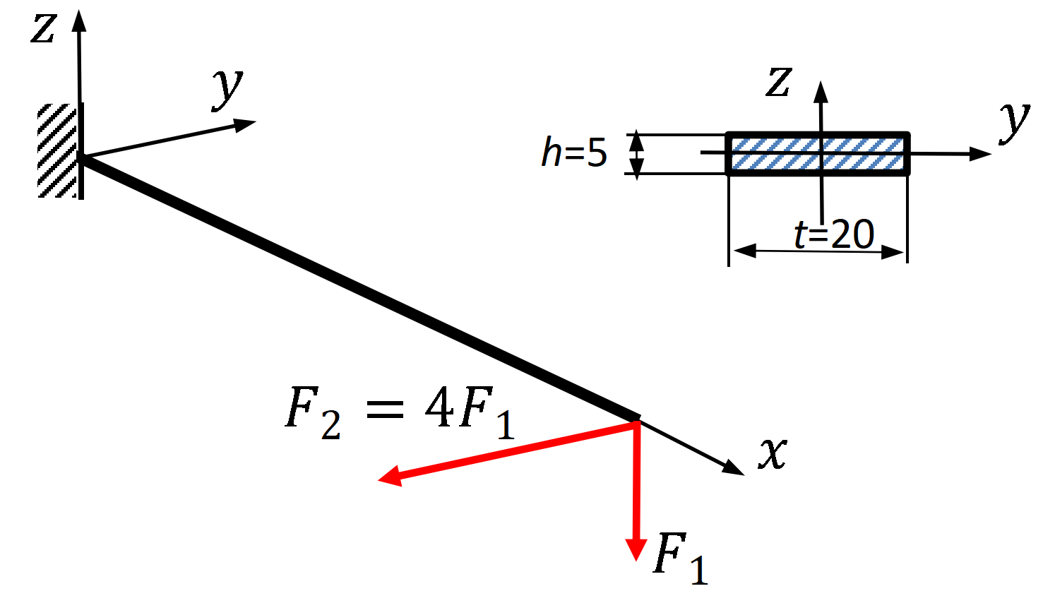
Example A straight cantilever is loaded as shown below. Its length is L = 200 m m L=200\,\mathit{mm} L = 200 mm 20 × 5 m m 20\times5\,\mathit{mm} 20 × 5 mm y y y z z z
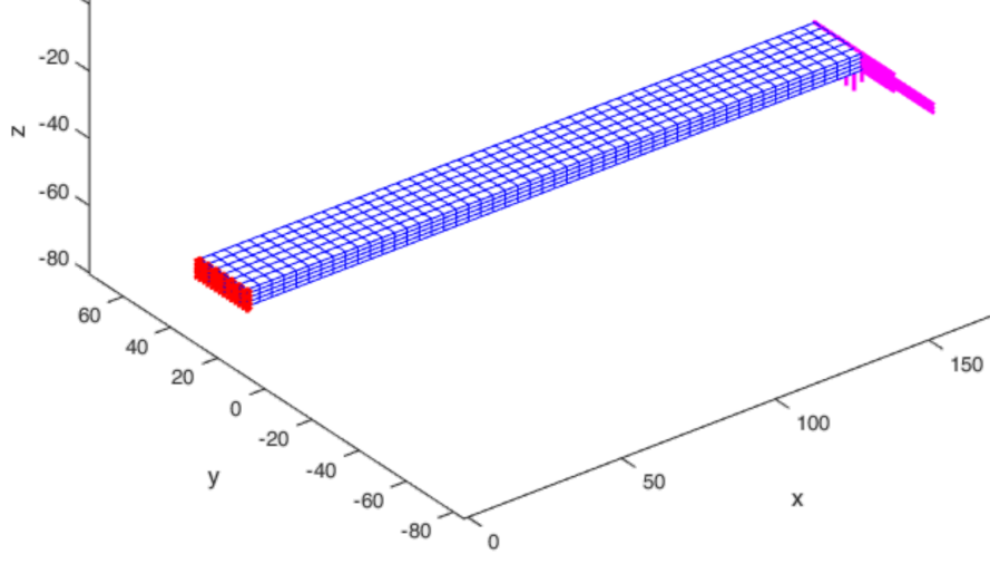
E = 2 × 10 5 M P a , ν = 0.3 , F 1 = 4000 N , F 2 = 4 F 1 . E=2\times10^5\,\mathit{MPa},\qquad\nu=0.3,\qquad F_1=4000\,\mathit N,\qquad F_2=4F_1. E = 2 × 1 0 5 MPa , ν = 0.3 , F 1 = 4000 N , F 2 = 4 F 1 . Figure 1. Cantilever geometry, cross-section and applied end loads. Dimensions are in millimetres.The 50 × 6 × 4 50\times6\times4 50 × 6 × 4
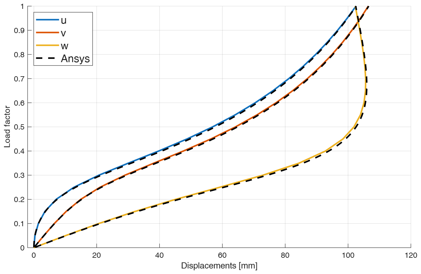
Figure 2. HEX8 mesh, constraints and end loading.The load-factor/displacement diagram compares the displacements of the centre of the loaded cross-section with ANSYS results.
Figure 3. Load factor versus displacements of the centre of the loaded cross-section [mm]; dashed curves show ANSYS results.
Figure 4. Deformed cantilever. Coordinates are in millimetres. Drag to rotate; Zoom is initially OFF. Reset view restores the initial camera.12
Stress plots Remark on stress plots. Although the stress components are calculated with respect to the global coordinate system, their representation on the deformed configuration is often more intuitive. For example, the σ x \sigma_x σ x
The stresses obtained directly from the Total Lagrangian constitutive relation are referred to the initial configuration. If stresses in the current configuration are required, they can be transformed to Cauchy stresses according to:
σ C = 1 J F S F T , \htmlClass{fea-math-bold-italic}{\boldsymbol{\sigma}}_C=\frac1J\htmlClass{fea-math-bold-italic}{\boldsymbol F}\htmlClass{fea-math-bold-italic}{\boldsymbol S}\htmlClass{fea-math-bold-italic}{\boldsymbol F}^T, σ C = J 1 F S F T , where S \htmlClass{fea-math-bold-italic}{\boldsymbol S} S σ \htmlClass{fea-math-bold-italic}{\boldsymbol{\sigma}} σ F \htmlClass{fea-math-bold-italic}{\boldsymbol F} F J = d e t ( F ) J=\mathop{\mathit{det}}(\htmlClass{fea-math-bold-italic}{\boldsymbol F}) J = det ( F ) Chapter 14 .
PREVIOUS SECTION ← 25.4. Fast program for the 20-node isoparametric hexahedral finite element NEXT SECTION 26.2. Isoparametric 20-node hexahedral finite element →