Chapter 24. Updated Lagrangian formulation, 3D isoparametric 2-node beam element

Hypotheses:

StrainSmall

DisplacementLarge

MaterialLinear

Timoshenko beam model.

Straight, prismatic, two-node isoparametric beam element. The element formulation follows the notation introduced in Section 23.3.

In the Updated Lagrangian formulation, the equilibrium configuration obtained at the end of load step $i$ becomes the reference configuration for load step $i+1$ . Therefore, the incremental displacements and stresses at the current load step are evaluated with respect to the previously deformed configuration.

The present formulation extends to 3D the Updated Lagrangian procedure introduced for the 2D case in Section 8.2.

The generalized strain vector is expressed in the local reference frame, using the notation introduced in Section 23.3.

\htmlClass{fea-math-bold-italic}{\boldsymbol{\varepsilon}}=\begin{Bmatrix}\varepsilon_0\\\beta_{\bar y}\\\beta_{\bar z}\\\kappa_{\bar x}\\\kappa_{\bar y}\\\kappa_{\bar z}\end{Bmatrix}.

The element nodal displacement vector in the local reference frame is:

\overline{\htmlClass{fea-math-bold-italic}{\boldsymbol u}}_{el}=\begin{Bmatrix}\bar u_1&\bar v_1&\bar w_1&\psi_{\bar x1}&\psi_{\bar y1}&\psi_{\bar z1}&\bar u_2&\bar v_2&\bar w_2&\psi_{\bar x2}&\psi_{\bar y2}&\psi_{\bar z2}\end{Bmatrix}^{T}.

For each load step, the element equations are written in the current local reference frame of the straight two-node beam element.

Generalized strains

Axial strain

The axial strain is evaluated from the exact change of element length:

\boxed{\varepsilon_0=\frac{\sqrt{(\bar v_2-\bar v_1)^2+(\bar w_2-\bar w_1)^2+(L-\bar u_1+\bar u_2)^2}}{L}-1}

where $L$ is the element length in the reference configuration of the current load step.

The corresponding current length is:

L_t=(1+\varepsilon_0)L.

Shear angles

Let the rotations of the normal to the deformed centroidal axis be:

\varphi_{\bar z}=\mathop{\mathit{arctan}}\left(\frac{\bar v'}{1+\bar u'}\right),

and

\varphi_{\bar y}=-\mathop{\mathit{arctan}}\left(\frac{\bar w'}{1+\bar u'}\right).

Using the sign convention established in Section 23.3,

\varphi_{\bar z}=\psi_{\bar z}+\beta_{\bar y},

while

\varphi_{\bar y}=\psi_{\bar y}-\beta_{\bar z}.

Therefore,

\boxed{\beta_{\bar y}=\mathop{\mathit{arctan}}\left(\frac{\bar v'}{1+\bar u'}\right)-\psi_{\bar z}}

and

\boxed{\beta_{\bar z}=\mathop{\mathit{arctan}}\left(\frac{\bar w'}{1+\bar u'}\right)+\psi_{\bar y}.}

For the two-node isoparametric element, the rotations vary linearly along the element. At the single Gauss point $\xi=0$ ,

\psi_{\bar y}(0)=\frac{\psi_{\bar y1}+\psi_{\bar y2}}{2},\qquad\psi_{\bar z}(0)=\frac{\psi_{\bar z1}+\psi_{\bar z2}}{2}.

The corresponding shear angles at the Gauss point are obtained directly from the nodal displacements and rotations.

{\beta }_{\bar y}\left( \xi\right) =\mathop{\mathit{arctan}}\left( \frac{{\overline{v}}_{2}-{\overline{v}}_{1}}{L+{\overline{u}}_{2}-{\overline{u}}_{1}}\right) -\left( \frac{1-\xi}{2}{{\psi }_{\overline{z}}}_{1}+\frac{1+\xi}{2}{{\psi }_{\overline{z}}}_{2}\right)

\mathit{and}

{\beta }_{\bar y}\left( 0\right) =\mathop{\mathit{arctan}}\left( \frac{{\overline{v}}_{2}-{\overline{v}}_{1}}{L+{\overline{u}}_{2}-{\overline{u}}_{1}}\right) -\frac{{{\psi }_{\overline{z}}}_{1}+{{\psi }_{\overline{z}}}_{2}}{2}

{\beta }_{\bar z}\left( \xi\right) =\mathop{\mathit{arctan}}\left( \frac{{\overline{w}}_{2}-{\overline{w}}_{1}}{L+{\overline{u}}_{2}-{\overline{u}}_{1}}\right) +\left( \frac{1-\xi}{2}{{\psi }_{\overline{y}}}_{1}+\frac{1+\xi}{2}{{\psi }_{\overline{y}}}_{2}\right) \, \, \, \, \, \, \mathit{and}\, \, \, \, \, \, \, {\beta }_{\bar z}\left( 0\right) =\mathop{\mathit{arctan}}\left( \frac{{\overline{w}}_{2}-{\overline{w}}_{1}}{L+{\overline{u}}_{2}-{\overline{u}}_{1}}\right) +\frac{{{\psi }_{\overline{y}}}_{1}+{{\psi }_{\overline{y}}}_{2}}{2}

Curvatures

In the present formulation, the curvatures are approximated by retaining the first-order terms:

\boxed{\kappa_{\bar x}=\frac{\psi_{\bar x2}-\psi_{\bar x1}}{L}}

\boxed{\kappa_{\bar y}=\frac{\psi_{\bar y2}-\psi_{\bar y1}}{L}}

\boxed{\kappa_{\bar z}=\frac{\psi_{\bar z2}-\psi_{\bar z1}}{L}.}

The second-order terms of the curvature expressions are neglected here. Their complete expressions and corresponding derivatives are presented separately in Addendum 24a.

This keeps the main development focused on the practical Updated Lagrangian algorithm, while the more complete curvature expressions can be consulted when required.

Deformation energy

The deformation energy of one beam element, expressed in the local reference frame, is:

U_{el}=\frac12\int_L\left[EA\varepsilon_0^2+GA_{\bar y}\beta_{\bar y}^2+GA_{\bar z}\beta_{\bar z}^2+GI_t\kappa_{\bar x}^2+EI_y\kappa_{\bar y}^2+EI_z\kappa_{\bar z}^2\right]d\bar x.

Using one Gauss integration point located at the element centre,

\xi_G=0,

the energy is evaluated as:

U_{el}\approx\frac L2\left[EA\varepsilon_0^2+GA_{\bar y}\beta_{\bar y0}^2+GA_{\bar z}\beta_{\bar z0}^2+GI_t\kappa_{\bar x}^2+EI_y\kappa_{\bar y}^2+EI_z\kappa_{\bar z}^2\right].

Element force vector and tangent stiffness matrix

The internal element force vector is obtained from the first derivative of the deformation energy:

\boxed{\overline{\htmlClass{fea-math-bold-italic}{\boldsymbol f}}_{el}=\frac{\partial U_{el}}{\partial\overline{\htmlClass{fea-math-bold-italic}{\boldsymbol u}}_{el}}}

and the tangent stiffness matrix from its second derivative:

\boxed{\overline{\htmlClass{fea-math-bold-italic}{\boldsymbol k}}_{el}=\frac{\partial^2 U_{el}}{\partial\overline{\htmlClass{fea-math-bold-italic}{\boldsymbol u}}_{el}^{\,2}}.}

$\varepsilon_i$ is the $i$ -th component of the generalized strain vector $\htmlClass{fea-math-bold-italic}{\boldsymbol{\varepsilon}}$ .

For each generalized strain component $\varepsilon_i$ , the corresponding contribution to the internal force vector contains its first derivative,

\frac{\partial\varepsilon_i}{\partial\overline{\htmlClass{fea-math-bold-italic}{\boldsymbol u}}_{el}},

whereas the tangent stiffness contribution contains both its first and second derivatives:

\frac{\partial\varepsilon_i}{\partial\overline{\htmlClass{fea-math-bold-italic}{\boldsymbol u}}_{el}}\left(\frac{\partial\varepsilon_i}{\partial\overline{\htmlClass{fea-math-bold-italic}{\boldsymbol u}}_{el}}\right)^T

and

\varepsilon_i\frac{\partial^2\varepsilon_i}{\partial\overline{\htmlClass{fea-math-bold-italic}{\boldsymbol u}}_{el}^{\,2}}.

The tangent stiffness matrix contains a material contribution, associated with the first derivatives of the generalized strains, and a geometric contribution, associated with their second derivatives.

{\overline{\htmlClass{fea-math-bold-italic}{\boldsymbol{f}}}}_{el}=L\left( EA{\varepsilon }_{0}^{\, }\frac{d{\varepsilon }_{0}^{\, }}{d{\overline{\htmlClass{fea-math-bold-italic}{\boldsymbol{u}}}}_{el}}+G{A}_{0\overline{y}}{\beta }_{0\overline{y}}^{\, }\frac{d{\beta }_{0\overline{y}}^{\, }}{d{\overline{\htmlClass{fea-math-bold-italic}{\boldsymbol{u}}}}_{el}}+G{A}_{0\overline{z}}{\beta }_{0\overline{z}}^{\, }\frac{d{\beta }_{0\overline{z}}^{\, }}{d{\overline{\htmlClass{fea-math-bold-italic}{\boldsymbol{u}}}}_{el}}+G{I}_{t}{\kappa }_{\overline{x}}^{\, }\frac{d{\kappa }_{\overline{x}}^{\, }}{d{\overline{\htmlClass{fea-math-bold-italic}{\boldsymbol{u}}}}_{el}}+E{I}_{\overline{y}}{\kappa }_{\overline{y}}^{\, }\frac{d{\kappa }_{\overline{y}}^{\, }}{d{\overline{\htmlClass{fea-math-bold-italic}{\boldsymbol{u}}}}_{el}}+E{I}_{\overline{z}}{\kappa }_{\overline{z}}^{\, }\frac{d{\kappa }_{\overline{z}}^{\, }}{d{\overline{\htmlClass{fea-math-bold-italic}{\boldsymbol{u}}}}_{el}}\right)

{\overline{\htmlClass{fea-math-bold-italic}{\boldsymbol{k}}}}_{el}=L\left[ EA\left( {\varepsilon }_{0}^{\, }\frac{{d}^{2}{\varepsilon }_{0}^{\, }}{d{\overline{\htmlClass{fea-math-bold-italic}{\boldsymbol{u}}}}_{el}^{2}}+\frac{d{\varepsilon }_{0}^{\, }}{d{\overline{\htmlClass{fea-math-bold-italic}{\boldsymbol{u}}}}_{el}}{\left( \frac{d{\varepsilon }_{0}^{\, }}{d{\overline{\htmlClass{fea-math-bold-italic}{\boldsymbol{u}}}}_{el}}\right) }^{T}\right) \, +\right. G{A}_{0\overline{y}}\left( {\beta }_{0\overline{y}}^{\, }\frac{{d}^{2}{\beta }_{0\overline{y}}^{\, }}{d{\overline{\htmlClass{fea-math-bold-italic}{\boldsymbol{u}}}}_{el}^{2}}+\frac{d{\beta }_{0\overline{y}}^{\, }}{d{\overline{\htmlClass{fea-math-bold-italic}{\boldsymbol{u}}}}_{el}}{\left( \frac{d{\beta }_{0\overline{y}}^{\, }}{d{\overline{\htmlClass{fea-math-bold-italic}{\boldsymbol{u}}}}_{el}}\right) }^{T}\right) +\, \, \, \, \, \, \,

\, G{A}_{0\overline{z}}\left( {\beta }_{0\overline{z}}^{\, }\frac{{d}^{2}{\beta }_{0\overline{z}}^{\, }}{d{\overline{\htmlClass{fea-math-bold-italic}{\boldsymbol{u}}}}_{el}^{2}}+\frac{d{\beta }_{0\overline{z}}^{\, }}{d{\overline{\htmlClass{fea-math-bold-italic}{\boldsymbol{u}}}}_{el}}{\left( \frac{d{\beta }_{0\overline{z}}^{\, }}{d{\overline{\htmlClass{fea-math-bold-italic}{\boldsymbol{u}}}}_{el}}\right) }^{T}\right) \, \, +G{I}_{t}\left( {\kappa }_{\overline{x}}^{\, }\frac{{d}^{2}{\kappa }_{\overline{x}}^{\, }}{d{\overline{\htmlClass{fea-math-bold-italic}{\boldsymbol{u}}}}_{el}^{2}}+\frac{d{\kappa }_{\overline{x}}^{\, }}{d{\overline{\htmlClass{fea-math-bold-italic}{\boldsymbol{u}}}}_{el}}{\left( \frac{d{\kappa }_{\overline{x}}^{\, }}{d{\overline{\htmlClass{fea-math-bold-italic}{\boldsymbol{u}}}}_{el}}\right) }^{T}\right) +

\, \, E{I}_{\overline{y}}\left( {\kappa }_{y}^{\, }\frac{{d}^{2}{\kappa }_{\overline{y}}^{\, }}{d{\overline{\htmlClass{fea-math-bold-italic}{\boldsymbol{u}}}}_{el}^{2}}+\frac{d{\kappa }_{\overline{y}}^{\, }}{d{\overline{\htmlClass{fea-math-bold-italic}{\boldsymbol{u}}}}_{el}}{\left( \frac{d{\kappa }_{\overline{y}}^{\, }}{d{\overline{\htmlClass{fea-math-bold-italic}{\boldsymbol{u}}}}_{el}}\right) }^{T}\right) \, \, \, \, \, \, \, \, +\, \, E{I}_{\overline{z}}\left. \left( {\kappa }_{\overline{z}}^{\, }\frac{{d}^{2}{\kappa }_{\overline{z}}^{\, }}{d{\overline{\htmlClass{fea-math-bold-italic}{\boldsymbol{u}}}}_{el}^{2}}+\frac{d{\kappa }_{\overline{z}}^{\, }}{d{\overline{\htmlClass{fea-math-bold-italic}{\boldsymbol{u}}}}_{el}}{\left( \frac{d{\kappa }_{\overline{z}}^{\, }}{d{\overline{\htmlClass{fea-math-bold-italic}{\boldsymbol{u}}}}_{el}}\right) }^{T}\right) \right] \, \, \, \, \, \, \, \, \, \, \, \, \, \, \, \, \,

The complete first and second derivatives of

\varepsilon_0,\quad\beta_{\bar y},\quad\beta_{\bar z},\quad\kappa_{\bar x},\quad\kappa_{\bar y},\quad\kappa_{\bar z}

with respect to $\overline{\htmlClass{fea-math-bold-italic}{\boldsymbol u}}_{el}$ are implemented in the MATLAB subprogram deriv.

\frac{d{\varepsilon }_{0}^{\, }}{d{\overline{\htmlClass{fea-math-bold-italic}{\boldsymbol{u}}}}_{el}}=\frac{1}{{L}^{2}}\left\{ \begin{matrix}-\left( L-{u}_{1}+{u}_{2}\right) \\{v}_{1}-{v}_{2}\\{w}_{1}-{w}_{2}\\0\\0\\0\\\left( L-{u}_{1}+{u}_{2}\right) \\-\left( {v}_{1}-{v}_{2}\right) \\-\left( {w}_{1}-{w}_{2}\right) \\0\\0\\0\end{matrix}\right\}

\frac{{d}^{2}{\varepsilon }_{0}^{\, }}{d{\overline{\htmlClass{fea-math-bold-italic}{\boldsymbol{u}}}}_{el}^{2}}=\frac{1}{{L}^{2}}\left[ \begin{matrix}1 & 0 & 0 & 0 & 0 & 0 & -1 & 0 & 0 & 0 & 0 & 0\\0 & 1 & & & & & & -1 & & & & \\0 & & 1 & & & & & & -1 & & & \\0 & & & & & & & & & & & \\0 & & & & & & & & & & & \\0 & & & & & & & & & & & \\-1 & & & & & & 1 & & & & & \\0 & -1 & & & & & & 1 & & & & \\0 & & -1 & & & & & & 1 & & & \\0 & & & & & & & & & & & \\0 & & & & & & & & & & & \\0 & & & & & & & & & & & \end{matrix}\right]

\frac{d{\beta }_{0\overline{y}}^{\, }}{d{\overline{\htmlClass{fea-math-bold-italic}{\boldsymbol{u}}}}_{el}}=\frac{1}{{L}^{2}}\, \left\{ \begin{matrix}-\left( {v}_{1}-{v}_{2}\right) \\-\left( L-{u}_{1}+{u}_{2}\right) \\0\\0\\0\\-{L}^{2}/2\\{v}_{1}-{v}_{2}\\L-{u}_{1}+{u}_{2}\\0\\0\\0\\-{L}^{2}/2\end{matrix}\right\}

\frac{{d}^{2}{\beta }_{0\overline{y}}^{\, }}{d{\overline{\htmlClass{fea-math-bold-italic}{\boldsymbol{u}}}}_{el}^{2}}=\frac{1}{{L}^{2}}\left[ \begin{matrix}\, 0 & -1 & 0 & 0 & 0 & 0 & \, 0 & 1 & 0 & 0 & 0 & 0\\1 & & & & & & -1 & \, & & & & \\0 & & & & & & & & \, & & & \\0 & & & & & & & & & & & \\0 & & & & & & & & & & & \\0 & & & & & & & & & & & \\0 & 1 & & & & & \, & -1 & & & & \\-1 & & & & & & 1 & \, & & & & \\0 & & & & & & & & \, & & & \\0 & & & & & & & & & & & \\0 & & & & & & & & & & & \\0 & & & & & & & & & & & \end{matrix}\right]

\frac{d{\beta }_{0\overline{z}}^{\, }}{d{\overline{\htmlClass{fea-math-bold-italic}{\boldsymbol{u}}}}_{el}}=-\frac{1}{{L}^{2}}\, \left\{ \begin{matrix}{w}_{1}-{w}_{2}\\0\\L-{u}_{1}+{u}_{2}\\0\\-{L}^{2}/2\\0\\-\left( {w}_{1}-{w}_{2}\right) \\0\\-\left( L-{u}_{1}+{u}_{2}\right) \\0\\-{L}^{2}/2\\0\end{matrix}\right\}

\frac{{d}^{2}{\beta }_{0\overline{z}}^{\, }}{d{\overline{\htmlClass{fea-math-bold-italic}{\boldsymbol{u}}}}_{el}^{2}}=-\frac{1}{{L}^{2}}\left[ \begin{matrix}0\, & \, 0 & 1 & 0 & 0 & 0 & \, 0 & \, 0 & -1 & 0 & 0 & 0\\0\, & & & & & & \, & \, & & & & \\-1 & & & & & & 1 & & \, & & & \\0 & & & & & & & & & & & \\0 & & & & & & & & & & & \\0 & & & & & & & & & & & \\0 & \, & -1 & & & & \, & \, & 1 & & & \\\, 0 & & & & & & \, & \, & & & & \\1 & & & & & & -1 & & \, & & & \\0 & & & & & & & & & & & \\0 & & & & & & & & & & & \\0 & & & & & & & & & & & \end{matrix}\right]

\frac{d{\kappa }_{\overline{x}}^{\, }}{d{\overline{\htmlClass{fea-math-bold-italic}{\boldsymbol{u}}}}_{el}}=\frac{1}{{L}^{\, }}\, \left\{ \begin{matrix}0\\0\\0\\-1\\0\\0\\0\\0\\0\\1\\0\\0\end{matrix}\right\}

\frac{d{\kappa }_{\overline{y}}^{\, }}{d{\overline{\htmlClass{fea-math-bold-italic}{\boldsymbol{u}}}}_{el}}=\frac{1}{{L}^{\, }}\, \left\{ \begin{matrix}0\\0\\0\\0\\-1\\0\\0\\0\\0\\0\\1\\0\end{matrix}\right\}

\frac{d{\kappa }_{\overline{z}}^{\, }}{d{\overline{\htmlClass{fea-math-bold-italic}{\boldsymbol{u}}}}_{el}}=\frac{1}{{L}^{\, }}\, \left\{ \begin{matrix}0\\0\\0\\0\\0\\-1\\0\\0\\0\\0\\0\\1\end{matrix}\right\}

\frac{{d}^{2}{\kappa }_{\overline{x}}^{\, }}{d{\overline{\htmlClass{fea-math-bold-italic}{\boldsymbol{u}}}}_{el}^{2}}={\htmlClass{fea-math-bold-italic}{\boldsymbol{0}}}_{12x12}

\frac{{d}^{2}{\kappa }_{\overline{y}}^{\, }}{d{\overline{\htmlClass{fea-math-bold-italic}{\boldsymbol{u}}}}_{el}^{2}}={\htmlClass{fea-math-bold-italic}{\boldsymbol{0}}}_{12x12}

\frac{{d}^{2}{\kappa }_{\overline{z}}^{\, }}{d{\overline{\htmlClass{fea-math-bold-italic}{\boldsymbol{u}}}}_{el}^{2}}={\htmlClass{fea-math-bold-italic}{\boldsymbol{0}}}_{12x12}

The exact axial strain itself is evaluated using the current element length. In the derivatives used to form the tangent quantities, however, the approximation

L_t\approx L

is adopted because the axial strain remains small:

\varepsilon_0\ll1.

This simplification leads to compact derivative expressions while preserving the accuracy required by the present formulation.

Updated Lagrangian procedure

The MATLAB implementation follows closely the 2D Updated Lagrangian algorithm presented in Section 8.2.

At each load step:

the equilibrium equations are solved for the incremental nodal displacements;
the nodal coordinates are updated;
the current element lengths are recomputed;
the element local reference frames are updated;
the auxiliary third nodes used to define the principal plane of each 3D beam element are updated;
the resulting configuration becomes the reference configuration for the next load step.

After updating the nodal coordinates,

x\leftarrow x+\mathit{\Delta} u,\qquad y\leftarrow y+\mathit{\Delta} v,\qquad z\leftarrow z+\mathit{\Delta} w,

the current length of every element is recalculated as:

\boxed{L_t=\sqrt{(x_2-x_1)^2+(y_2-y_1)^2+(z_2-z_1)^2}.}

This explicit update is used in the subprogram updt.

Update of the local reference frame

In 3D, each two-node beam element uses an auxiliary third node in order to define the principal plane of the cross-section. The coordinates of these auxiliary nodes are stored in the table nd3.

The orientation of this third node must be updated after every load step.

For sufficiently small incremental rotations, a first-order incremental rotation matrix may be used. However, higher accuracy is obtained by retaining the second-order terms of the incremental rotation matrix, as discussed in Section 21.1.

Let the incremental nodal rotations of the current beam element be:

\varphi_x,\qquad\varphi_y,\qquad\varphi_z.

The corresponding second-order incremental rotation matrix is denoted by

\htmlClass{fea-math-bold-italic}{\boldsymbol R}_i.

{\htmlClass{fea-math-bold-italic}{\boldsymbol{R}}}_{i}=\left[ \begin{matrix}1-\frac{1}{2}\left( {\varphi }_{y}^{2}+{\varphi }_{z}^{2}\right) & {-\varphi }_{z}+\frac{1}{2}{\varphi }_{x}{\varphi }_{y} & {\varphi }_{y}+\frac{1}{2}{\varphi }_{z}{\varphi }_{x}\\{\varphi }_{z}+\frac{1}{2}{\varphi }_{x}{\varphi }_{y} & 1-\frac{1}{2}\left( {\varphi }_{z}^{2}+{\varphi }_{x}^{2}\right) & -{\varphi }_{x}+\frac{1}{2}{\varphi }_{y}{\varphi }_{z}\\\htmlClass{fea-math-bold-italic}{\boldsymbol{-}}{\varphi }_{y}+\frac{1}{2}{\varphi }_{z}{\varphi }_{x} & {\varphi }_{x}+\frac{1}{2}{\varphi }_{y}{\varphi }_{z} & 1-\frac{1}{2}\left( {\varphi }_{x}^{2}+{\varphi }_{y}^{2}\right) \end{matrix}\right]

With the convention used in the subprogram updt, the accumulated transformation is updated according to:

\boxed{\htmlClass{fea-math-bold-italic}{\boldsymbol R}\leftarrow\htmlClass{fea-math-bold-italic}{\boldsymbol R}_i^T\htmlClass{fea-math-bold-italic}{\boldsymbol R}.}

The auxiliary third node is then updated consistently with the new element orientation.

MATLAB program

The MATLAB implementation for the 3D Updated Lagrangian formulation follows the same general structure as the 2D program presented in Section 8.2.

The main subprograms are:

gen_ex2.m — Example 2 input data and mesh generation;
stiff — assembly of the tangent stiffness matrix and internal force vector;
deriv — first and second derivatives of the generalized strains;
updt — update of nodal coordinates, element lengths and local reference frames.

The exact axial strain is used directly in the numerical calculations, while the simplified derivative expressions described above are used in the tangent formulation.

The MATLAB package includes both deriv.m and deriv_corrected.m. The routine deriv_corrected.m implements the complete curvature expressions presented in Addendum 24a.

MATLAB3D Updated Lagrangian beam programDownload ZIP

Example 1

The first example is the large-displacement 3D cantilever problem presented in Section 22.2.

The same material, geometric and loading data are used.

To reproduce the reference solution closely, the Updated Lagrangian analysis is performed using 50 load steps.

The algorithm presented in Section 22.2 provides a highly accurate reference solution for this example. Consequently, using fewer load steps in the UL formulation leads to larger, although still small, errors.

**Figure 1.** Example 1. Deformed cantilever configuration.

Example 2

A very flexible cantilever beam is considered:

L=100\ \mathit{mm},

with rectangular cross-section

6\times9\ \mathit{mm},

Young's modulus

E=1000\ \mathit{MPa},

and Poisson's ratio

\nu=0.3.

The free end is loaded by:

Y=50\ \mathit{N},\qquad Z=50\ \mathit{N},\qquad M_x=3500\ \mathit{Nmm}.

The beam is discretized with 30 elements and the load is applied in 40 load steps.

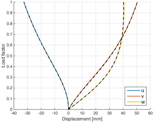
The MATLAB results are compared with ANSYS results and show very good agreement.

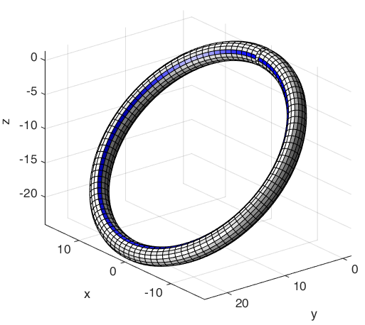
Figure 2. Example 2. Deformed cantilever configuration; the end at the origin is clamped.

**Figure 3.** Example 2. Load–displacement comparison: solid lines — MATLAB; dashed lines — ANSYS.

ANSYSExample 2 — ANSYS macroDownload ZIP

Example 3

An initially straight cantilever beam lies along the global $x$ -axis and is clamped at $x=0$ . Its rectangular cross-section has dimensions $2\,\mathit{mm}$ in the $y$ -direction and $3\,\mathit{mm}$ in the $z$ -direction. $E=2\times10^5\,\mathit{MPa}$ . The beam is loaded at its free end by $X=-150\,\mathit N$ , $Y=50\,\mathit N$ , $Z=75\,\mathit N$ , $C_x=15000\,\mathit{Nmm}$ , $C_y=0$ , $C_z=20000\,\mathit{Nmm}$ .

The beam length is:

L=100\ \mathit{mm},

Figure 4. Example 3. Deformed cantilever configuration; the end at the origin is clamped.

ANSYS does not reach the prescribed final load for this example. The solution stops at 35% of the total load:

X=-52.5\ \mathit{N},\qquad Y=17.5\ \mathit{N},\qquad Z=26.25\ \mathit{N},

C_x=5250\ \mathit{Nmm},\qquad C_y=0,\qquad C_z=7000\ \mathit{Nmm}.

At this load level, the maximum displacements are:

Method	u [mm]	v [mm]	w [mm]
Section 22.2, finite-difference method	−68.835	59.471	44.004
Present UL formulation, 50 load steps	−69.738	59.970	43.286
ANSYS	−69.343	59.581	43.859

The agreement between the three solutions is very good.